YOLIN Optimisation program
OMNEC Optimisation program
Theory with examples.
Practical Design
Boom corrections
Losses in elements
Errors in computer simulations
Since some 20 years it has been possible to perform accurate computer simulations of antennas. Very highly optimised yagis may have bandwidths well below 1%, so for such antennas it is essential to take systematic errors into account when translating computer simulations into real antennas.In 1975, Chen and Cheng published a six element optimised design - maximum gain using six elements only, with no concern on anything else, such as bandwidth, impedance or spurious lobes. In these early simulations the systematic errors are quite large, a direct building after the theoretical dimension does not give any useful antenna.
For a yagi antenna the first order systematic errors are of two kinds. For simplicity, assume all elements are made from rods (or tubes) of only one diameter. One correction is due to end effects, and it is a constant that has to be added to all elements. In older simulations, due to the neglect of the currents flowing through the end capacitors, this constant may be in the order of 10 mm for a 10 mm tube on 144 MHz. To this should be added another correction that is proportional to the element length - and the size depends on the method used. For a yagi antenna, all elements are close to one half wavelength, so the second correction also becomes nearly a constant and therefore the two corrections may be replaced by a single correction term, equal for all elements.
To determine the correction in going from theory to the real world, the radiation pattern is the important factor. An error in element lengths, equal for all elements is in the first order a shifting of the design frequency. By comparing the real radiation pattern with the theoretical pattern, one can determine the frequency shift and use that to correct all the elements. Note that since only lengths, not positions are wrong, the pattern is only similar, not equal to the calculated one. See The Optimum 6 Element Yagi Antenna, an article that was published in UKW Berichte / VHF communication 1981/1982. Note also that the reference is for the method only. The Chen Cheng design is not a particularly good design, probably because the element positions and lengths were not varied simultaneously during the optimisation process.
Comparisons between theoretical and experimental patterns give a good insight in the systematic errors of the calculations. If you have the radiation pattern in the E plane it is trivial to calculate the directive gain of a yagi antenna by integration. The reason is that the current distribution on each element is close to the current distribution on a half wave dipole, so the E pattern of a yagi can be taken as the array factor for stacking half wave dipoles. The field in an arbitrary direction then is the product of the E-plane radiation pattern and the pattern for a dipole. To get the real gain, ohmic losses have to be included afterwards.
For an evaluation of antenna gain figures by measurement of the E plane pattern look at Measurement of radiation patterns. Nordic VHF Meeting, Öland 970606
Since the directive gain of an antenna is the far field in the forward direction divided by the average far field it is possible to obtain antennas with maximum gain by looking for designs that have minimum for the average far field, provided that the radiation pattern is properly normalised. Rather than looking for maximum of one function (gain) one looks for the minimum of the sum of the squares of many simultaneous functions - radiated power is the square of the electric field. In this way convergency is obtained, and true maximum gain yagis can be designed within the simulation model chosen. For a detailed description see Computer Design of Very High Gain Yagi Antennas. Here the method applied is a computer program from about 1972 by Kuo and Strait, that uses piecewise linear current functions on the elements, and that does not take end capacitances into account. Nevertheless this method can be used to construct real antennas with very good performance, and I have used it to design my present 4x14 element antenna. The computer program YOLIN is easy to use, but for large arrays the computing speed is slow. This program takes ohmic losses into account in an approximate way that works reasonably well only if the design frequency is 144MHz.
My previous antenna, BSZ09.YAG, 9 elements for stacking at 3.7m, YO format, was designed the same way with YOLIN, and it was my first test of the Kuo and Strait program. When I had found the corrections (-15mm) as described in The Optimum 6 Element Yagi Antenna, I was happily surprised (after adding a well designed balun) that the feed impedance was accurately 50 ohms, exactly as calculated. This antenna, which was mounted on wooden booms is a good test case for checking various computer simulation software.
Modifying NEC2 for optimisation
The 9 element design for stacking at 3.7m, BSZ09.NEC described above, and corrected by 15mm as found by experiment was used as input to NEC2. When running NEC2 one has to specify the number of segments to use for each wire (element). The figures below show the result from NEC2 with 3 to 39 segments for each element. You may look at the data in numerical form.
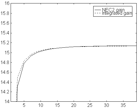
Fig 1. Gain vs number of segments per element. Original NEC2 for a 9 element yagi with 9mm elements on 144 MHz. The gain is calculated in two ways. The solid line is gain as obtained directly from NEC2, calculated from the absolute value of the far field in the forward direction. The dotted line is the gain as calculated from the far field in the forward direction divided by the average far field. The dotted line includes ohmic losses.
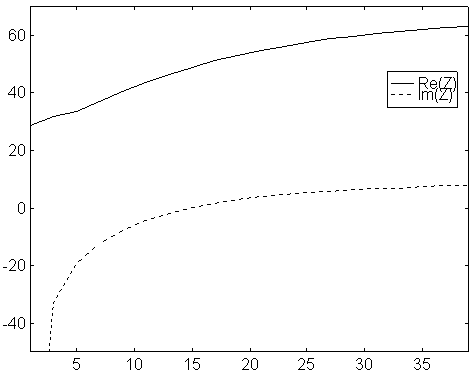
Fig2. Feed point impedance vs number of segments per element. Original NEC2 for a 9 element yagi with 9mm elements on 144 MHz. Solid line is real part and dotted line is imaginary part.
The results produced by NEC2 depend too much on the segment length for NEC2 to be a really nice model to optimise yagis in.
By adding a few lines in the NEC source code, filling the array BI(I) in the routine WIRE with a slightly modified element radius, adding a new array with the unmodified radius for use by the routine LOAD, the first order errors can be compensated. The modified radius, BI(I) = RAD * ( 0.94 + 2.7 * SEG / WL), where SEG is the segment length and WL is the wavelength. In my mind, this way of absorbing errors in the calculation of matrix elements makes good physical sense, as long the element diameters are within reasonable limits ( 3 - 15 mm on 144 MHz).
With the modified version of NEC, the calculation results are much less depending on the number of segments. See the diagrams below or the numerical data.
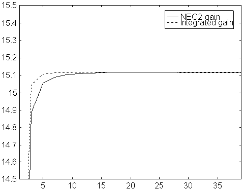
Fig 3. Gain vs number of segments per element. Modified NEC2 for a 9 element yagi with 9mm elements on 144 MHz. The gain is calculated in two ways. The solid line is gain as obtained directly from NEC2, calculated from the absolute value of the far field in the forward direction. The dotted line is the gain as calculated from the far field in the forward direction divided by the average far field. The dotted line includes ohmic losses.
.
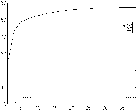
Fig 4. Feed point impedance vs number of segments per element. Modified NEC2 for a 9 element yagi with 9mm elements on 144 MHz. Solid line is real part and dotted line is imaginary part.
Note that, with the modified NEC2, the gain as calculated from the theoretical radiation pattern is constant within 0.005dB from 3 to 39 segments, and that the imaginary part of the feed point impedance is constant. For the purpose of using the model to optimise antennas, this is very valuable. The optimisation can be performed with only 3 or 5 segments per element - and still the same result is obtained as if 15 segments had been used!!!
The modified NEC2 will probably allow the design of more critical antennas. In the original NEC2, the imaginary part of the element impedance changes when the segment length is changed - and the segment lengths vary with the element lengths - and therefore slightly different corrections have to be added to long and short elements. From a practical point of view this is unacceptable. With the modified NEC2, a constant correction, equal for all elements should lead to a real world design with a radiation pattern that is very accurately the same as the calculated pattern. If the pattern is accurate, then gain, G/T and everything else is as in the model - and the real antenna is the optimum antenna for the optimisation criteria used.
When selecting the constants 0.94 and 2.7, I used not only the 9mm diameter 9 element design, I also looked at the 5mm diameter, 10 element design, BSZ10.NEC 10 elements for overstacking. This antenna uses 5 mm elements, while the 9 element design uses 9mm elements. The number 0.94 is a compromise, but I do not have information enough to select a more elaborate expression that would be more accurate. Look here for more details on comparisons of original NEC2 with the modified NEC2.
If you like to make your own designs with the modified NEC2 optimisation program, you should find everything you need here: Modified NEC2 Optimisation Program This package is not as easy to use as YOLIN, but it is more accurate. It is also not limited to conventional yagis. Any structure that can be represented by thin wires can be optimised although problems may occur with convergency in some cases. Note that this program is at an early stage, and may contain various bugs.
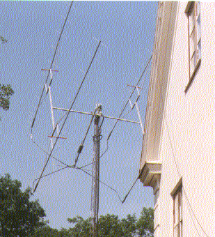
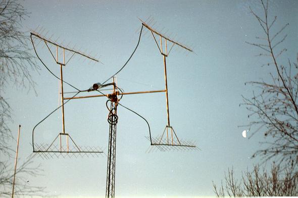
Since August 1993 I have been using a 4x14 element antenna designed for 50 ohms at 144.1MHz with YOLIN. Here is a photo (44k). showing the antenna and part of my house.Here is another photo (34k) showing antenna details better. (Thank you Kevin) This design was experimentally calibrated for a 50mm boom tube by changing all elements by an equal amount until the impedance was correct at 144.1MHz as outlined above, and described more in detail Practical Design of Very High Gain Yagi Arrays Look here Simulation by NEC2 of Experimental Antenna Adjustment. The element lengths differ by 15.5 millimeters between the two methods. Unfortunately I do not know the free space element lengths. With the elements mounted above a 50mm boom tube in such a way that the air gap is 14mm, the correct lengths are 7mm shorter than the theoretical obtained from YOLIN, and 8.5mm longer than the theoretical ones from NEC2.
To SM 5 BSZ Main Page