Linrad, two channel reception,
noise cancelling, antennas phasing.

Linrad has been for a long time a software of choice for experimenters and those who need a program which is actually SDR laboratory. One of Linrad features which is rarely used is its two coherent channels reception. Possibility of processing signals from two locked in phase receivers opens the door to the fascinating realm of antennas phasing, beamforming, diversity reception and noise cancelling. Recently a new Phasing window was introduced to Linrad. This paper is a simple manual to it.

1. Linrad Phasing window.

Phasing window is an extension for Polarization window (Fig. 1). You may also understand it as a “translator” since it translates parameters understandable in the world of two crossed antennas of vertical and horizontal polarization (VHF) to parameters typical for the domain of HF antennas phasing, namely: amplitude (or: gain) balance and phase shift between two channels.

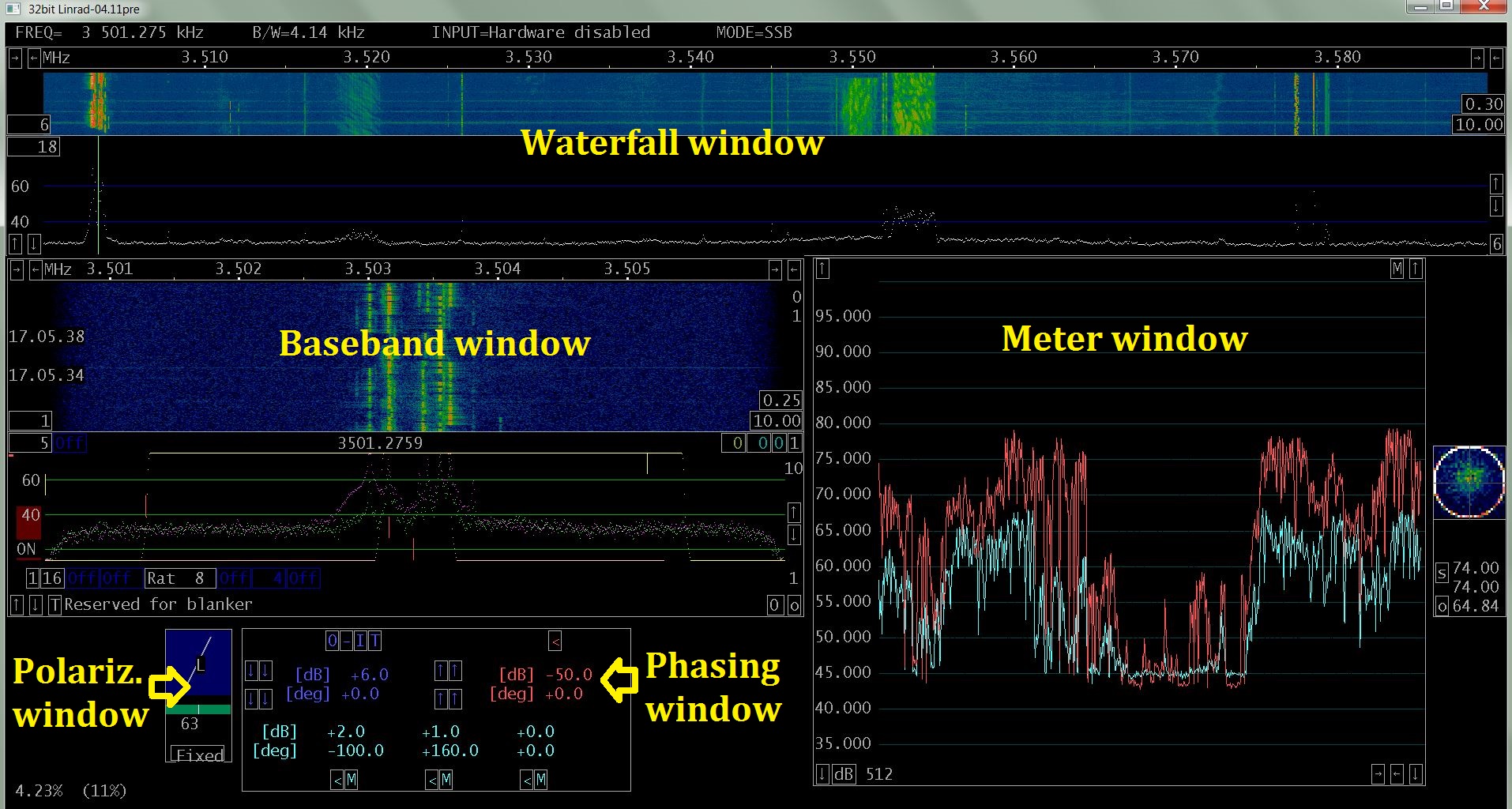
Fig. 1. Windows in Linrad.

When a new Linrad installation is set up for the first time the polarization menu will appear (Fig 2.). Toggle H to enable / disable Phasing window. Recommended D value is Man (for: “Manual”). Parameters B and C are provided for compensation of difference in cable lengths and gain balance.

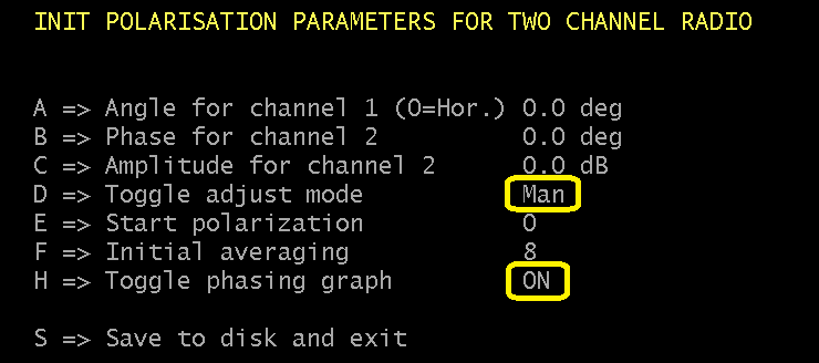
Fig 2. Polarization parameters.

You may always return to this menu from the normal processing screen by pressing X followed by D.

Phasing window (Fig. 3) is divided in three sections, each of them has its own color.

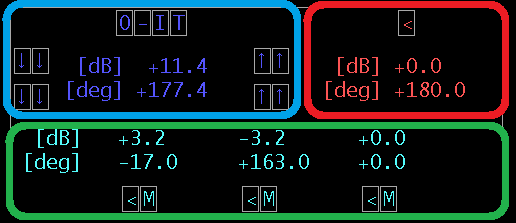
Fig. 3. Sections of Phasing window

The blue section elements:

1. Numerical values of actual gain balance and phase shift.

These are the actual values of channel 2 gain balance and phase shift (delay) in reference to channel 1. When positive: channel 2 gain is greater than gain of channel 1 and channel 2 is delayed.

2. Arrow buttons.

The inner buttons are for slow and outer buttons for fast decrease / increase of gain balance and phase shift.

3. “O” button.

Orthonormal transformation. Changes the sign of gain balance and adds 180 degrees to phase shift (e.g. pair -3 dB, +38 degrees becomes +3 dB, -142 degrees. More to be explained below in Appendix A)

4. “-“ button.

Changes the sign of phase shift (e.g. +38 degrees becomes -38 degrees).

5. “I” button.

Inversion of phase. 180 degrees is being added (e.g. +38 degrees turns into -142 degrees).

6. “T” button.

Individual channel toggle. Toggles the gain balance between -50 dB (channel 2 attenuated) and +50 dB (channel 1 attenuated).

The green section elements:

There are three memories for gain & phase pairs. You remember the present value of gain and phase (as seen in the blue section) by clicking on “M” button. You apply the content of the memory (send it to the program) when clicking on respective “<” button.

The red section elements:

Provided for numerical input from keyboard. Click on gain or phase value, type your own value followed by “Enter”, click on “<” button to apply.

2. How to use Phasing window.

2.1. Noise cancelling.

The original function of Polarization window and its advanced adaptive function is to trace automatically changing amplitude and phase of incoming signals in EME communication and to provide the best possible combination of signal received in two channels.

Since adaptive function has priority over the manual settings please remember to keep “Adapt / Fixed” button of Polarization window in its “Fixed” value. It is a default value here unless otherwise stated.

It may be also wise to keep the “AGC” OFF. This will allow you to hear in changes and difference of signal levels.

2.1.1. Noise cancelling (manual).

Let us say that except of our signal of interest there is an interfering signal S in the passband of receiver. Two antennas and two coherent SDR channels enable cancelling of one specific unwanted signal or noise. To accomplish this following conditions must be met:

– the interfering signal S must be “heard” (i.e. received) by each of the antennas,

– we must adjust the gain balance to achieve the same amplitude of S in both channels,

– there should be 180 degrees phase shift between S in both channels.

With these assumptions fulfilled adding two channels leads to subtracting interfering signal. If, say, amplitude in channel 2 has been adjusted not exactly to S value, but to 0.99 of S we will get 0.01 (i.e. -40 dB) of S still present in the sum of two channels. The level of other signals present in the passband, including our signal of interest, is a consequence of a choice of unique phase and gain adjusted for cancelling of S.

Here is a defeated noise visible in a Baseband graph:

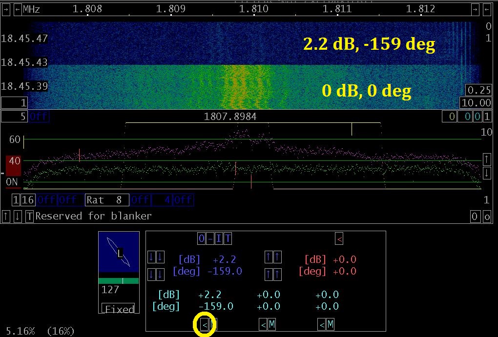
Fig. 4. Manual noise cancelling.

At 18.45.43 I’ve applied new set of gain balance and phase shift: 2.2 dB, -159 deg (notice the “<” button at picture bottom), the old values were: 0 dB, 0 deg. Nothing found below noise, but satisfaction is my award :-) .

How have I come to values 2.2 dB and -159 deg? In following steps as shown in Meter window (Fig 5):

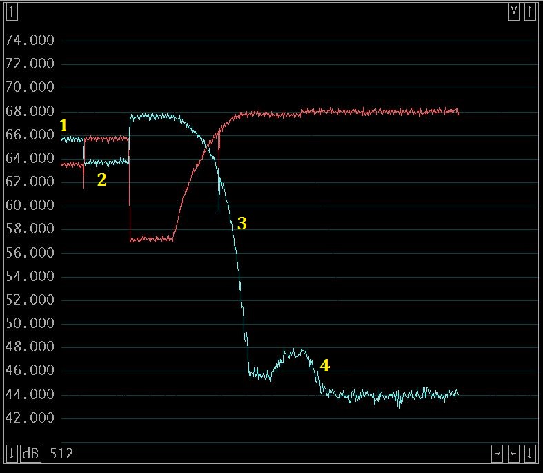
Fig. 5. Manual noise cancelling - steps.

In this moment we pay attention only to a green trace on the graph. We want to make it as low as possible.

The procedure of manual noise reduction comprises following steps:

- Click button “T”,

- Step 1 – measurement of noise level in channel 1, result 66 dB,

- Click button “T”,

- Step 2 – noise measurement in channel 2, 64 dB, that is 2 dB less,

- Entering values: 2 dB, 0 degrees in red section, applying with red “<”,

- Step 3 – fast adjusting of phase down to approx. -160 degrees,

- Step 4 – fine adjustment of phase and gain.

The final result is 24 dB reduction of noise.

2.1.2. Noise cancelling (semi-automatic).

Now we will use the adaptive function of Polarization window.

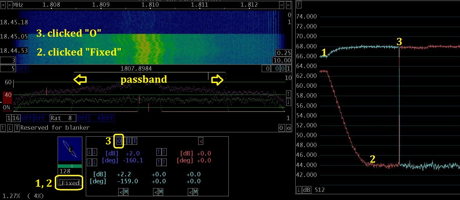
Fig. 6. Noise cancelling, adaptive.

Since adaptive polarization function searches for phase and gain parameters to maximize the strongest signal in a passband we will employ it to the strong noise which you can see on the waterfall of Baseband window in Fig. 6.

The procedure is following:

- Step 1 – toggle the “Adapt / Fixed” button to enter into adaptive function,

- Step 2 – after the red trace in a Meter window stabilizes return to “Fixed” value,

- Step 3 – click on the “O” button.

Noise is not heard anymore. Here we got also 24 dB reduction of noise. The same as in manual procedure.

Sometimes we have two signals of a similar strength competing in a passband. Or a useful signal is too strong to let the adaptive function work effectively on noise. In such a case a simple approach may help: narrowing the passband of a filter and / or tuning to the interfering signal / noise alone.

After Linrad finds the magic gain and phase:

- switch to “Fixed” mode,

- click on “O” button (in this moment interference is gone),

- adjust filter width,

- tune precisely to your signal.

This is the way I’ve worked with the situation in Fig. 7. What you see now is a passband of 2,7 kHz. It was only 600 Hz wide when Linrad was busy in adaptive mode.

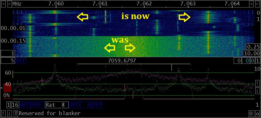
Fig. 7. Narrowing the filter.

2.2. Stereo diversity reception.

This is the kind of reception in which detected signal from each antenna / channel is provided as “stereo” to the headphones. Our brains can effectively process such a pair of coherent signals sometimes even better than software does.

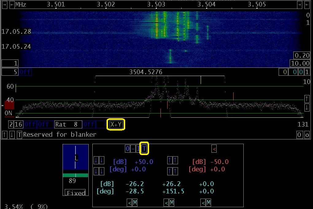
Fig. 8. Stereo diversity reception.

To benefit of this kind of reception (and to experience a pleasure of tracing signals which are wandering from one ear to the other) you need to:

- activate “X+Y” button in the Baseband window,

- click once or twice on a “T” button in Phasing window (the blue “Gain” value shall be either +50 dB or -50 dB),

- should you be unhappy with volume balance between audio channels, you’ll have to adjust levels in the Windows sound devices properties (you get there through right click on a “speaker” icon in task bar)

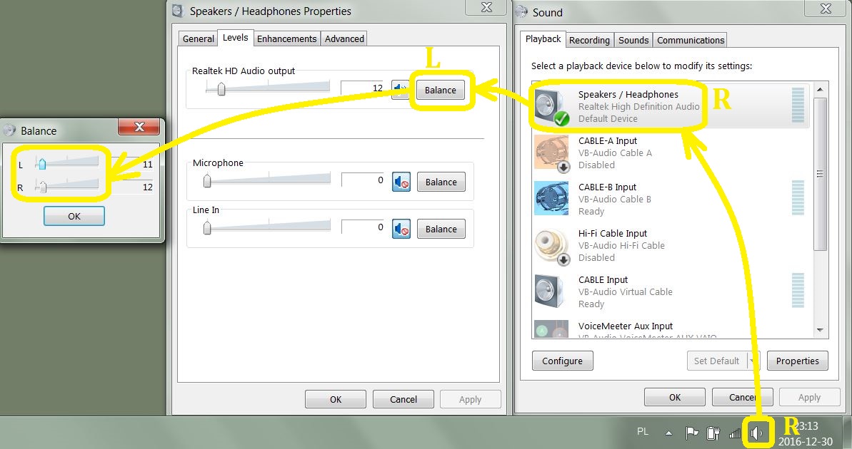
Fig. 9. Stereo balance adjusting,
R = right click, L = left click

2.3. Separating two stations on one frequency.

When two stations transmit on the same frequency you may apply following technique:

- extract stronger of them either in manual or in semi-automatic way described above in point 2,

- click on “X+Y” button in the Baseband window (Fig. 10),

- with “Fixed” value of “Adaptive Polarization” use “O” to swap audio channels (Fig. 10).

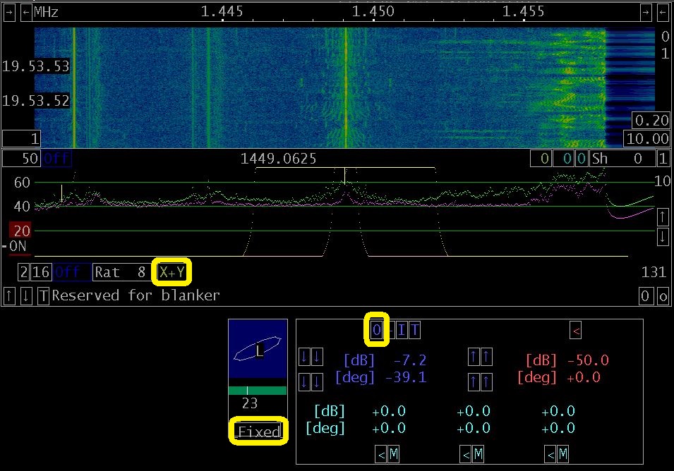
Fig. 10. Separation of two stations on the same frequency.

In this method Linrad routes strongest signal to one audio channel, and the rest of the passband content (all minus strongest signal) to another one. Stereo balance adjustment may be useful here. Be ready to see huge differences between gain level in two channels when distant and nearby stations occupy the same frequency (Fig 11).

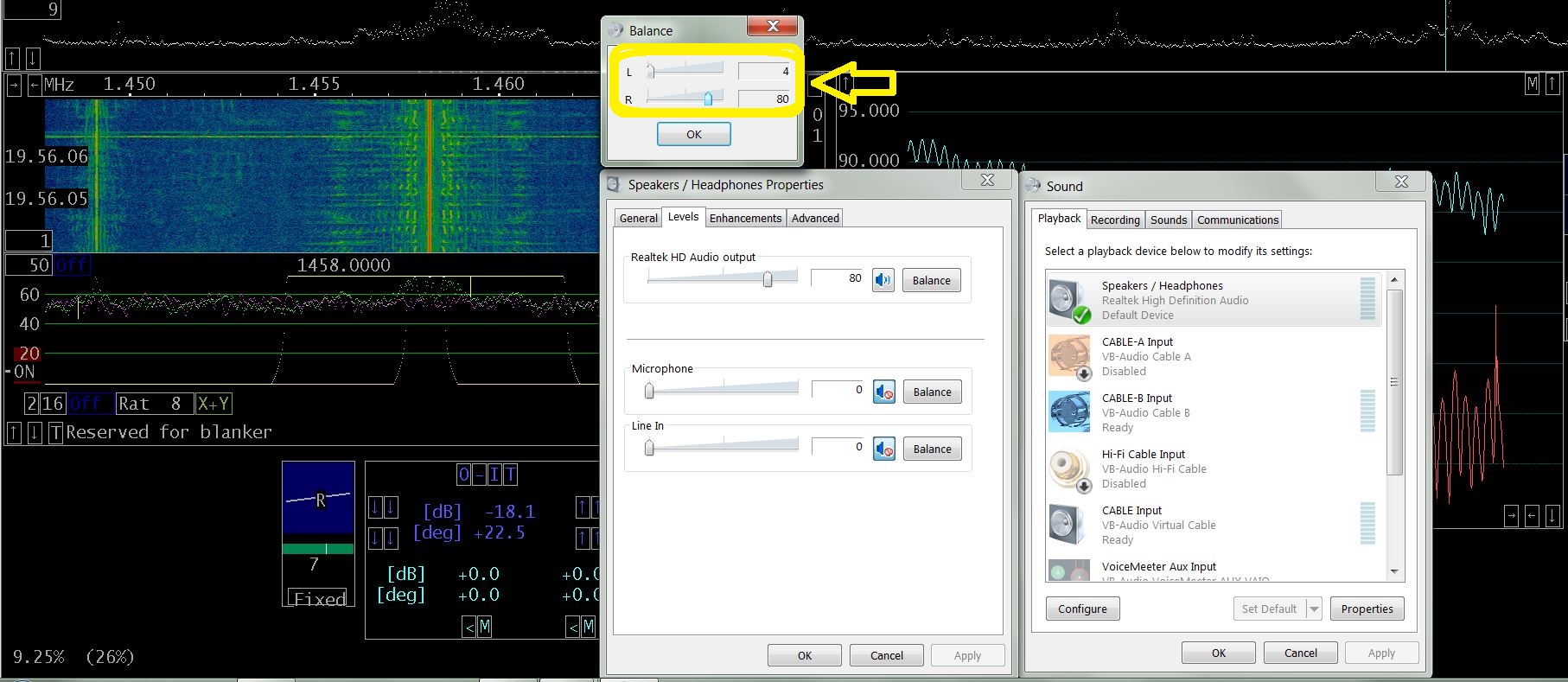
Fig. 11. Position of sliders for L and R audio of distant and nearby stations.

You will find an example of similar method in one of Leif’s videos: https://www.youtube.com/watch?v=TgEEZJuQoQ0 (begins at 22:10). Please notice that in this video Polarization window is in “Adapt” mode all the time. In such a case toggling “O” button is purposeless.

Leif’s version may be more adequate when stronger station signal is not stable.

2.4. Directional arrays, maximizing Signal-to-noise ratio.

All the above applications of Linrad are rather forgiving in terms of choice of antennas (please refer to Appendix D and Useful Links, p. 2 for details). It is not so with 2 element directional arrays which are usually made of 2 identical antennas in a friendly environment. What makes an environment friendly? Flat ground of uniform electrical properties, and lack of metal object in close vicinity. For instance my array is situated several meters from metal roofs. It makes it completely useless in terms of directivity. But I can still enjoy effective noise cancelling, nice stereo diversity and stations separation.

Fig. 12. Example of two vertically
oriented receiving loops in end-fire setup.

Depending on phase shift between its elements an array of phased antennas may have quite different patterns (Fig. 13).

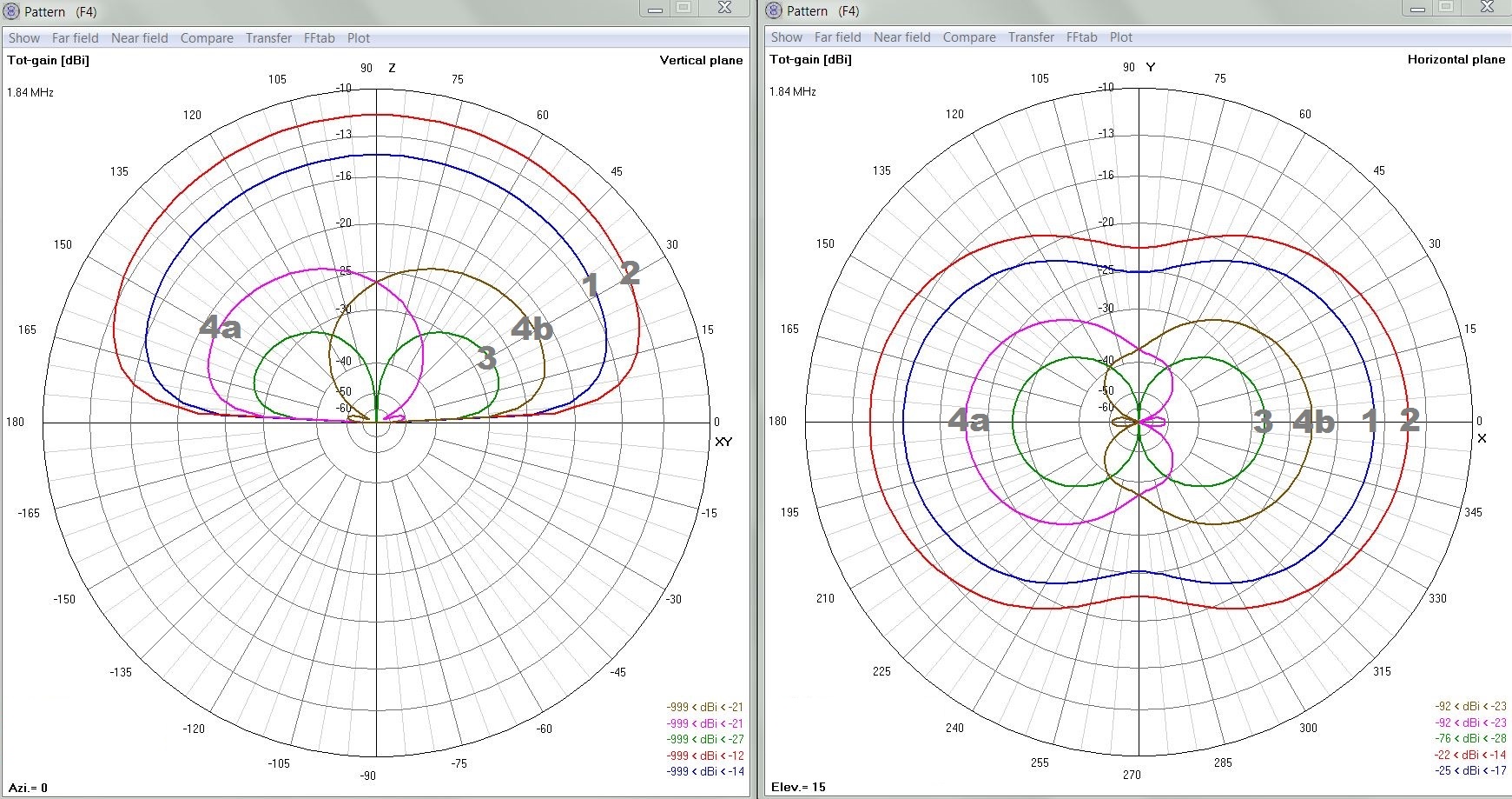
Fig. 13 End-fire array patterns.

Explication for Fig. 13:

1. Individual loop.

Following are two loops added with phase shift of:

2. 0 degrees (additive mode).

3. 180 degrees (bi-directional mode).

4a. and 4b. 180 degrees +/ -20 degrees (directional mode).

(20 degrees is a time delay between antennas translated to phase shift for a given frequency, see Useful links, Phasing of antennas)

Directional mode setups 4a and 4b provide best RDF (receiving directivity factor), i.e. they give chance for best signal-to-noise ratio (signal level dropdown between patterns 1 and 4 doesn’t matter on lower HF). They have also good front-to-back ratio. Chavdar Levkov’s, LZ1AQ, Receiving Phased Array and Mark Bauman’s, KB7GF, Shared Apex Loop Array make use of these properties of end-fire arrays.

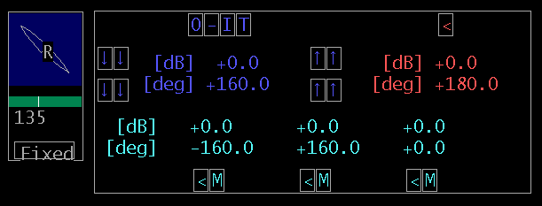
Fig 14. Phasing window with phase shift values fit for end-fire array.

You will easily notice that Phasing window is quite handy for operating end-fire array:

- individual loops are toggled with “T” button,

- additive mode entered from 3^rd green memory,

- bi-directional mode applied either by red “<” button or through phase inversion button “I“

- directional modes entered from 1^st and 2^nd green memories, swapped by “-“ button.

2.5. Radio direction finding.

Imagine we have an array which exhibits deep null and this null is steerable with gain balance and phase shift between the elements of the array. Let the pairs: azimuth & elevation will be in bi-unique correspondence to pairs: gain balance & phase shift.

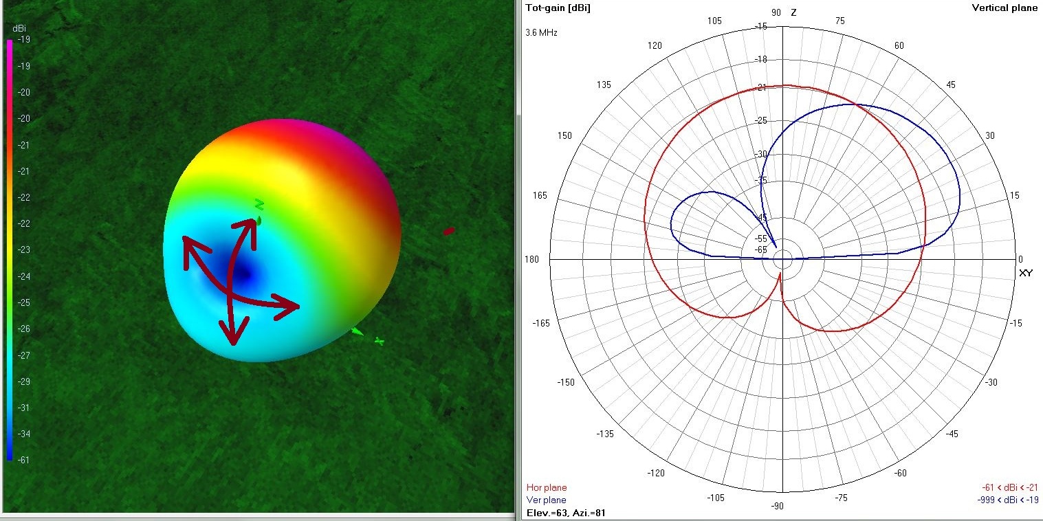
Fig 15. Direction finding.

Linrad may find inter-channel phase shift and gain balance of null (either in manual or adaptive/automatic way, see p. 2.2.). Through one-to-one mapping we may translate gain and phase to angles of azimuth and elevation.

In my exercises with antennas modeling I’ve come to conclusion that it is possible to build a combo:
- HF directional array, and in the same time,
- pretty precise direction finding system (0-360 degrees azimuth & 0-90 degrees elevation).

What is needed for this:
- 4 small antennas,
- 4-channel SDR,
- software preprocessor reducing the number of channels to 2,
- Linrad.

This could be reduced to:
- 4 antennas,
- small hardware - a box in the field with step attenuators and combiners
- box at home (controller),
- 2-channel SDR,
- Linrad.

Building it? Maybe… One day…

Appendix A.

Orthonormal transformation in Linrad.

This mysterious expression is a key to understanding Linrad automatic phasing feature. Do not be afraid. I’m not going to make things more complicated. In a minute or two all things will turn clear and understandable.

Please refer to Leif’s page Linrad Support: The Polarisation Graph (see Useful Links below). I will quote Leif here:

Linrad will combine the two RF channels by use of an orthonormal transformation. (…) The two RF signals  IN₁ and IN₂ are combined to give two output signals like this:

A * IN₁ + B * IN₂ 

A * IN₂ - B * IN₁ 

Let S be the strongest signal in the passband. We do not care here whether it is wanted signal or interfering signal. Important thing is that S is present in both: IN₁ and IN₂.

Adaptive function of Polarization window adjusts automatically parameters A and B to get S maximized on one of its outputs and minimized on the other one. This second output contains all the signals of a passband less S.

Following functional schematic may help to understand how these two outputs of Polarization window are routed. This schematic is valid only for “Fixed” value of “Fixed/Adapt” switch.

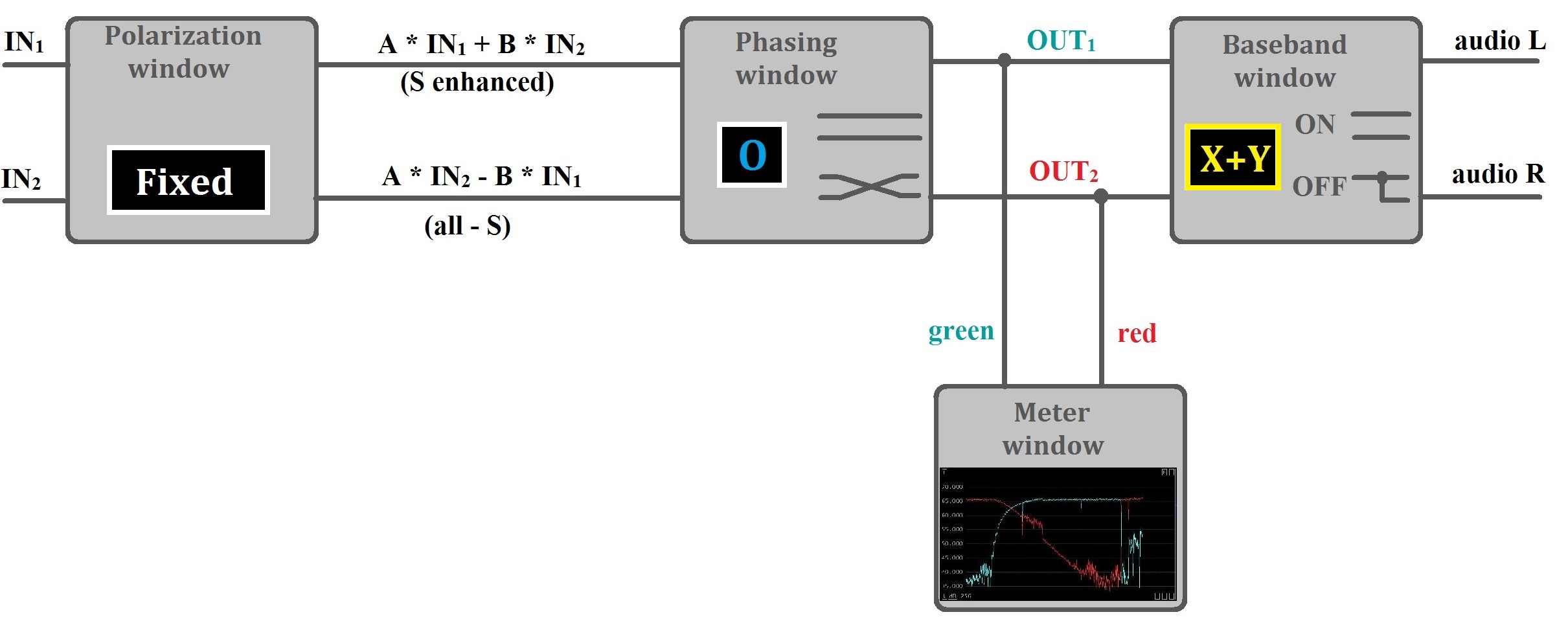
Fig. 16. Functional block diagram.

Example 1.

Let us say we have already come through the following steps:

- “Adapt” function has found optimum values of parameters A and B,

- clicking on the button we switched to “Fixed” mode

- “O” button has been tapped

- “X+Y” is ON.

We can hear now in the headphones:

- all signals less S in left audio channel,

- S enhanced in right audio channel.

Example 2.

We toggled “T” button, amplitude balance has been set to  -50 dB value. That means parameter B = 0.

Buttons values:

- “O” button has not been touched,

- “X+Y” is ON.

This time we can hear decoded IN₁ in left ear and IN₂ in right ear.

The Meter window is showing green IN₁ and red IN₂.

We may swap the channels in two ways: clicking either on “T” or on “O”.

You may return now to points 2.1. (noise cancelling), 2.2 (stereo diversity) and 2.3 (separating) to check whether this functional diagram works.

Please remember that the above schematic is valid only with “Fixed” value of polarization function. Toggling it to “Adapt” will result in restoring regular Linrad behavior.

For those who are hungry for more scientific approach: see Useful links, Orthonormal transformation in Linrad.

Appendix B.

Orthonormal transformation and array pattern.

Let us assume that we use Linrad for phasing of a pair of vertical loops in end-fire setup and our goal is cancelling interfering signal coming from 38 degrees elevation and 0 degrees azimuth angles.

Let adaptive function of Linrad find optimum values:

- gain balance between channels 0 dB,

- phase shift -14 degrees.

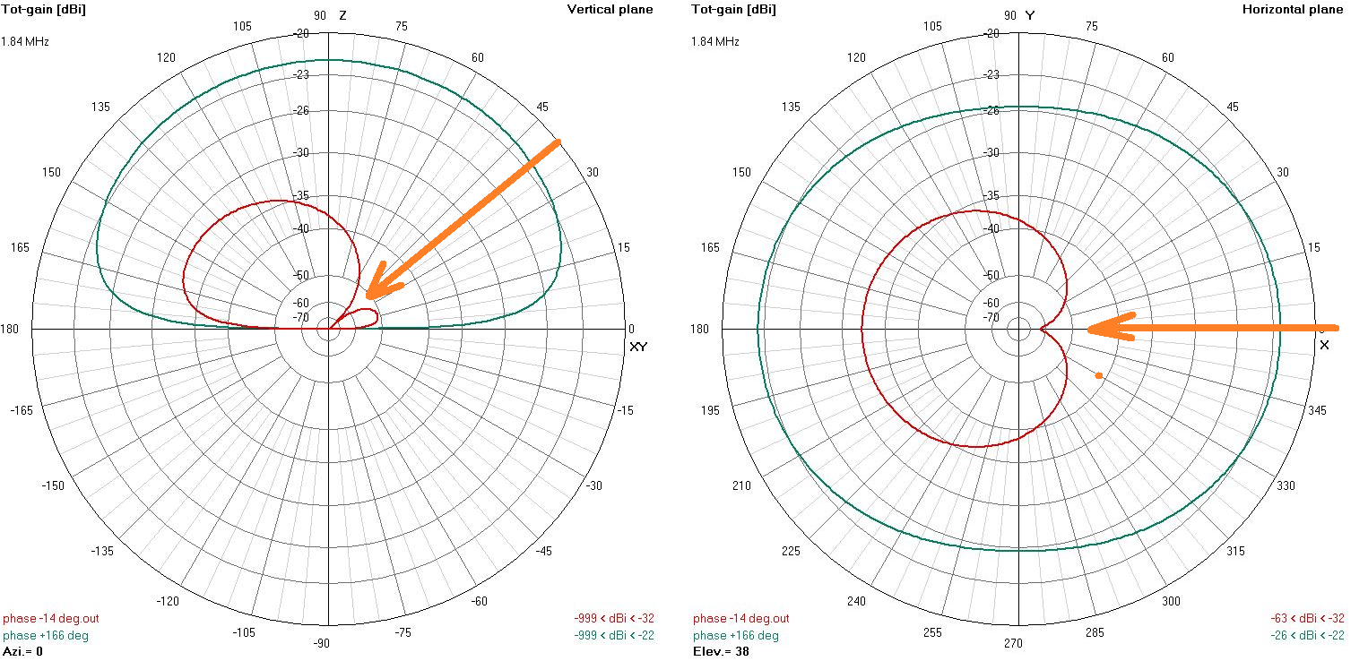
Fig. 17. Orthonormal transformation, patterns.

When these values are applied the null of the red pattern absorbs the interfering signal and we may listen to the rest of the signals according to red pattern response to them.

The green pattern is related to the red one by the virtue of orthonormal transformation.

Phase shift for green is: -14 + 180 = + 166 degrees.

Gain balance for green is equal -1 * 0 = 0 dB.

In response of green pattern our interfering signal is maximized.

Colors of the patterns are chosen to fit the colors of Meter window traces.

With “X+Y” button ON you have signals from both arrays: green and red, present in respective audio channels (left and right).

Appendix C.

Wideband recordings.

There is one feature extremely useful for those who want to experiment with phasing. It is wideband recording. Recording of several minutes of 100kHz wide part of crowded amateur radio band brings much material for future analysis.

Of course you may be satisfied by your phasing approach and skills in the real time. But replaying recordings provides unique possibility for repetitive listening. You may always choose piece of recordings with especially interesting noise or interference and set it in loop mode to be repeated endlessly.

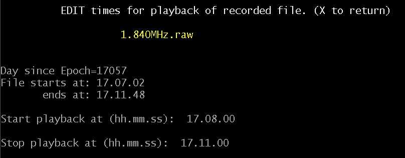
Fig. 18. Setting file playback parameters.

Both recording and playback control are initiated from the keyboard. S is for recording, F for setting beginning and end of replayed part of recording.

If you don’t have a dual channel receiver you may try Linrad with Leif’s recorded file available here: http://www.sm5bsz.com/linuxdsp/demo/demhf2.htm.

Recently I’ve started to listen to a chosen minutes of JT65 and JT9 transmissions. I try to find setup with the best signal-to-noise. This is real beam-forming exercise. There is no difference between such a rehearsal and beam-steering in real time. Even with my imperfect array I’ve succeeded to decode several stations which were not otherwise heard by individual antennas.

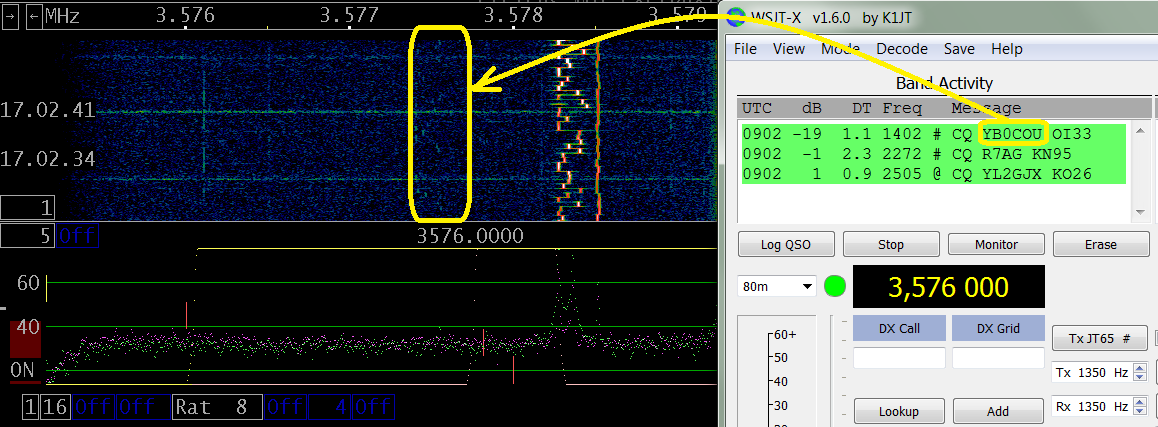
Fig 19. Indonesian station received in Eastern Europe on 80 meters (December, 17 UTC)

Appendix D.

Antennas for noise cancelling.

Sometimes you will meet opinions that only main reception antenna matters and the second antenna (noise sensor) could be any antenna with any localization. That is definitely not true.

First: signal from second antenna is added to signal from main antenna on equal rights. If it is buried in all kinds of noise you will let this noise in to your radio. Linrad will cancel only 1 specific interfering signal. The crowd of them will reach your ears. So keep both of your antennas far from sources of noise.

Second: Keep a proper distance between the antennas. Optimum is a quarter wavelength on a band of interest. As you see on Fig. 20 and 21 changing inter-channel phase shift from 0 to 180 degrees allows to null out any signal incoming from elevations 0 – 90 degrees. Elevation angle of a cancelled signal on Fig. 20 is ~73 degrees. Another 180 degrees of phase shift between the channels and we have swept whole hemisphere. For each every direction of incoming interference there is a “black hole” (or, rather “blue hole”, see Fig. 21) in array pattern, there is only a puzzle of finding the right phase shift.

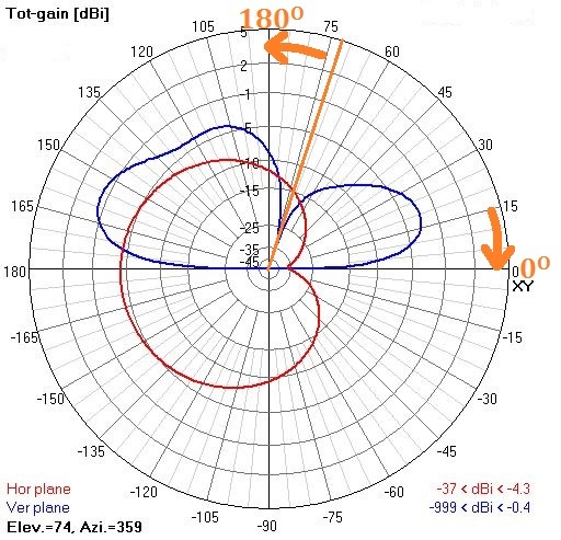
Fig. 20. Two phased antennas ¼ wavelength far from each other.

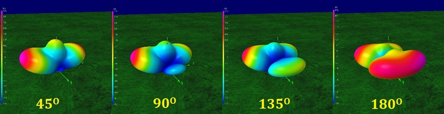
Fig. 21. 3D pattern of 2 phased antennas ¼ wavelength far from each other. Yellow numbers indicate phase shift between the channels.

If the distance is too big (one wavelength and more), there are too many sharp nulls, so finding and maintaining them may be difficult (Fig. 22). Far distant antennas form an array that is not easy steerable.

Fig. 22. Pattern of 2 phased antennas 3 wavelengths distant from each other.

Searching for proper gain balance and phase shift is actually equivalent to changing the pattern of 2 element array. In the case of noise cancelling it is difficult to call it beam-forming. It is rather null-forming, i.e. we try to form a null (as deep as possible) in the direction of arrival of unwanted, interfering signal.

Appendix E.

Phasing: Analog vs. SDR.

As far as I know they are three analog ways to adjust phase shift when adding signals picked up by antennas:

- using cable delay line (just like in KB7GF Shared Appex Loop Array),

- with electronic delay line (like in LZ1AQ Receiving Phased Array)

- with different phasers / noise cancellers / signal enhancers.

All of them deal with summing up in the RF front end. The digital solution (2 channel coherent SDR) moves the point of summing up signals from the front end to the PC and software.

Provided we use the same antennas in both cases (analog and digital) we will get the same results. I've compared front-to-back ratio when listening to several MW stations using:

- two loops => NCC-1 noise canceller

- two loops => 2 channel Afedri => PC & Linrad.

Got very similar level of interference cancelling.

The advantage of digital solution is its “adaptive” option. The software finds the best combination of gain balance / phase shift and saves me tweaking the knobs of canceller.

What may be interesting for some, there is also orthonormal transfomation present in process of analog noise cancelling. For instance toggling at once two switches in NCC-1 noise canceller (Fig. 23):

- swapping inputs (1),

- and applying phase invertion, i.e. adding 180 degrees to one of the channels (2)

is equivalent to clicking on “O” button in Linrad which results in swapping green and red orthonormal signals to software output.

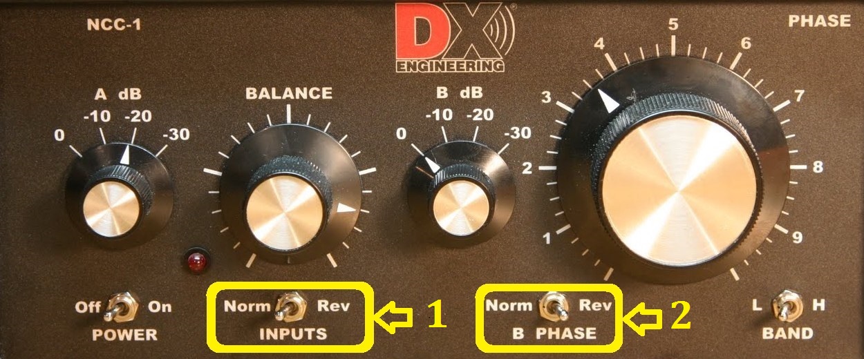
Fig. 23. DXE NCC-1 Phase Controller.

Useful links

1. Linrad.

Leif Asbrink, SM5BSZ, Linrad for newcomers
http://www.sm5bsz.com/linuxdsp/usage/newco/newcomer.htm

Gaëtan Horlin, ON4KHG Linrad Installation & Configuration User Guide
http://www.nitehawk.com/w3sz/Linrad%20Installation%20&%20Configuration%20User%20Guide%20-%20V1-0.pdf

2. Orthonormal transformation in Linrad.

Leif Asbrink, SM5BSZ, What is Polarisation ? Signals v.s. Noise
http://www.sm5bsz.com/polarity/poltheor.htm

Leif Asbrink, SM5BSZ, Linrad Support: The Polarisation Graph
http://www.sm5bsz.com/linuxdsp/run/polgr.htm

3. Stereo diversity reception (with audio recordings).

Tom Rauch, W8JI, Diversity Receiver and Transmission
http://www.w8ji.com/polarization_and_diversity.htm

Chavdar Levkov, LZ1AQ, Diversity Reception with a Modified SDR Receiver and Small Active Antennas
https://www.lz1aq.signacor.com/docs/dr/deversity-reception.htm

4. Phasing of antennas.

Chavdar Levkov, LZ1AQ, Receiving Phased Array with Small Electric or Magnetic Active Wideband Elements. Experimental Performance Evaluation
http://www.lz1aq.signacor.com/docs/phased-array/2-ele_phased_array11.pdf

Mark Bauman, KB7GF, Introducing the Shared Apex Loop Array
http://www.arrl.org/files/file/QEX_Next_Issue/Sep-Oct_2012/Bauman_QEX_9_12.pdf

5. Receiving Directivity Factor (RDF).

Tom Rauch, W8JI, Receiving basics
http://www.w8ji.com/receiving_basics.htm

Tom Rauch, W8JI, How Low-Noise Receiving Antennas Really Work
http://www.w8ji.com/receiving.htm

6. Antennas modeling.

Arie Voors, NEC based antenna modeler and optimizer
http://www.qsl.net/4nec2/?

Hardware used

1. Antennas.

Two Wellbrook ALA100LN Loops.

2. SDR.

Afedri AFE822x SDR-Net (Dual Channel).

3. Noise canceller.

DX Engineering NCC-1 Receive Antenna Variable Phasing Controller.

© Piotr Hewelt, SP2BPD

Additional proofreading - Marcin Marciniak, SP5XMI

January 1, 2017